WELL LOG EXERCISE SOLUTIONS

You can find our solutions to the well exercises below. Though we are happy with these solutions, or they would not be posted on the site, you should recognize that these solutions also represent matters of opinion that are based on the models we have chosen to build our interpretations from; remember "beauty is in the eye of the beholder" and not neccessarily the ultimate "truth"!

We also created a movie showing the evolution of a clastic sequence with incised valley fill utilizing the well logs used in these exercises. (you will need to have a QuickTime movie player in order to view the movie). Click on image to view the movie and use the left and right arrows on the keyboard to move backward and forward throught the movie (click here for a smaller-version). This movie gives a sense of the geological reasoning behind the well log interpretations that have been provided.

EXERCISE 1 Solution

• A segmented .pdf image of the cross-section with the solution to Exercise 1 can be printed, assembled and taped (PRINT-a-EX1-X-SEC).
• A complete .pdf image of the cross-section with the solution to Exercise 1 that can be printed as one image or segmented (PRINT-b-EX1-X-SEC).
• You can also view the solution file as a .jpg image (VIEW-EX1-X-SEC).
• All the well logs (from left to right W-1, W-2, W-3) were placed side-by-side and aligned with the top correlation marker (dotted line at the top of each well log).
• For each of the SP curves (the right trace) the areas of the curve with the "0" or low SP values are inferred to represent shale, while high SP values are inferred to represent sand, i.e. those values further from center line.
• The adjacent well logs are correlated on the basis of similarly shaped curves, by drawing a boundary surface under each correlatable interval. 
• On each of the well logs shale is colored green and sand yellow.
• You can review the data sheet sheet at the bottom of the x-section solution file for more precise values.
  

EXERCISE 2 Solution

• A .pdf image of the cross-section representing the solution to Exercise 2 can be printed, assembled and taped (PRINT-A-EX2-X-SEC).
• A complete .pdf image of the cross-section with the solution to Exercise 2 that can be printed as one image or segmented (PRINT-B-EX2-X-SEC).
• You can also view the solution file as a .jpg image (VIEW-EX2-X-SEC).
• All the well logs (from left to right W-1, W-2, W-3, etc.) were placed side-by-side and aligned with the top correlation marker (dotted line at the top of each well log).
• For each of the SP curves (the right trace) the areas of the curve with the "0" or low SP values are inferred to represent shale, while high SP values are inferred to represent sand, i.e. those values further from center line.
• On each of the well logs shale is colored green and sand yellow.
• The adjacent well logs are correlated on the basis of similarly shaped curves, by drawing a boundary surface under each correlatable interval. 
• The cross-section is divided into parasequences and the system tracts are identified within each parasequence.
• The transgressive surfaces were indentified first. These surfaces coincide with thin intervals of winnowed sediment that are produced as the sea transgresses across the underlying sediments. Thus the inferred transgressive surfaces are thin intervals that show a slight increase in grain size over thin shale intervals that may in turn overlie blocky sands. The transgressive surface is often indicated on the SP by an increase in grain size and a coincidental local increase in resistivity which matches carbonate cementation.
• The Maximum Flooding Surfaces (mfs's) of each parasequence was interpreted next. On the well logs these surfaces are interpreted to coincide with the occurrence of shale (kicks on the logs with the lowest SP values) just beneath sections that coarsen upward (i.e., the SP values increase, exhibiting a vertical funnel shape on the SP log). Three parasequences (each parasequence being enveloped by mfs) were identified and were labelled from the base up as A, B, and C.
• The sequence boundary (SB) on the cross-sections was the final surface identified. This was picked at the base of the channel sands (incised valley fill). A massive boxcar trend in log character was inferred to represent the channel fill of incised valleys and this fill was correlated to adjacent well logs.
• For each parasequence the total sand content in feet (utilize the middle log scale) was estimated while utilizing the middle of the log to mark sand body boundaries and triangles to record changes in grain size within each parasequence). The values were recorded in a spreadsheet.
• Based on the mfs surfaces and the identified channels, the systems tracts for each of the well logs (LST, TST, and HST) were identified.  Channel sands were interpreted to represent a Lowstand Systems Tract which was incised into the underlying Highstand Systems Tract, and is overlain by Transgressive System Tract deposits.  Where no channels were present, the mfs were utitilized to identify the HST (the deposits above the mfs) and the TST (the deposits below the mfs).
• The final step should be to write up an analysis describing your conclusions based on your interpretation of the depositional setting and the evolution of each parasequence.
• You can review the data sheet sheet at the bottom of the x-section solution file for more precise values.
  

EXERCISE 3 Solution

• Three .pdf images of the cross-sections represeting the solution to this exercise can be printed, assembled and taped (PRINT-X-SEC-A, PRINT-X-SEC-B, PRINT-X-SEC-C).
• You can also view and /or print the solution files as .jpg images (VIEW-X-SEC-A, VIEW-X-SEC-B,VIEW-X-SEC-C).
• Three well cross-sections were created: two parallel to strike and the third in the dip direction (see base map). The sequence stratigraphy of the sediments in the sections was interpreted using the cross-sections and the associated maps you created should illustrate your interpretations.
• All the well logs (from left to right W-1, W-2, W-3, etc.) were placed side-by-side and aligned with the top correlation marker (dotted line at the top of each well log).
• For each of the SP curves (the right trace) the areas of the curve with the "0" or low SP values are inferred to represent shale, while high SP values are inferred to represent sand, i.e. those values further from center line.
• On each of the well logs shale is colored green and sand yellow.
• The adjacent well logs are correlated on the basis of similarly shaped curves, by drawing a boundary surface under each correlatable interval. 
• The cross-section is divided into parasequences and the system tracts are identified within each parasequence. The Maximum Flooding Surfaces (mfs's) of each parasequence was identified first. On the well logs these surfaces are interpreted to coincide with the occurrence of shale (kicks on the logs with the lowest SP values) just beneath sections that coarsen upward (i.e., the SP values increase, exhibiting a vertical funnel shape on the SP log). Three parasequences (each parasequence being enveloped by mfs) were identified and were labelled from the base up as A, B, and C.
• The transgressive surfaces were indentified next. These surfaces coincide with thin intervals of winnowed sediment that are produced as the sea transgresses across the underlying sediments. Thus the inferred transgressive surfaces are thin intervals that show a slight increase in grain size over thin shale intervals that may in turn overlie blocky sands. The transgressive surface is often indicated on the SP by an increase in grain size and a coincidental local increase in resistivity which matches carbonate cementation.
• The sequence boundaries (SB) on the cross-sections were the final surfaces identified. These were picked at the base of the channel sands (incised valley fill). A massive boxcar trend in log character was inferred to represent the channel fill of incised valleys and this fill was correlated to adjacent well logs.
• For each parasequence the total sand content in feet (utilize the middle log scale) was estimated while utilizing the middle of the log to mark sand body boundaries and triangles to record changes in grain size within each parasequence). The values were recorded in the spreadsheet.
• Based on the mfs surfaces and the identified channels, the systems tracts for each of the well logs (LST, TST, and HST) were identified.  Channel sands were interpreted to represent a Lowstand Systems Tract which was incised into the underlying Highstand Systems Tract, and is overlain by Transgressive System Tract deposits.  Where no channels were present, the mfs were utitilized to identify the HST (the deposits above the mfs) and the TST (the deposits below the mfs).
• The final step should be to write up an analysis describing your conclusions based on your interpretation of the depositional setting, the evolution of each parasequence and the sand isopach maps.
• You can review the data sheet sheet at the bottom of each x-section solution file for more precise values.

EXERCISE 4 Solution

• A cross-section representing a potential solution to this exercise can be viewed on the .pdf file that can be accesses via the thumbnail and/or the.gif file from the link provided below. This solution to this exercise can be printed from either the .pdf and .jpg figures provided.

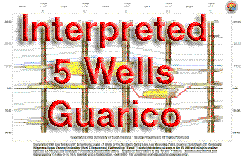
• As an alternative the above .pdf file this cross section can also be viewed by clicking on the link to a large .jpg file of the 5 Well Section Interpreted which provides the same solution to this exercise seen on the .pdf file.
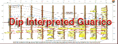
• For each of the SP curves (the right trace) the areas of the curve with the "0" or low SP values are inferred to represent shale, while high SP values are inferred to represent sand, i.e. those values further from center line.
• On each of the well logs shale is now colored brown and sand yellow.
• The adjacent well logs are correlated on the basis of similarly shaped curves, by drawing a boundary surface under each correlatable interval. 
• The cross-section is divided into parasequences and the system tracts are identified within each parasequence.  
• The Transgressive Surfaces (TSs) of each parasequence was identified first. These surfaces coincide with thin intervals of winnowed sediment that are produced as the sea transgresses across the underlying sediments. Thus the inferred transgressive surfaces are thin intervals that show a slight increase in grain size over thin shale intervals that may in turn overlie blocky sands. The transgressive surface is often indicated on the SP by an increase in grain size and a coincidental local increase in resistivity which matches carbonate cementation.
• The Maximum Flooding Surfaces (mfs's) of were identified next. On the well logs these surfaces are inferred to coincide with the occurrence of shale (kicks on the logs with the lowest SP values) just beneath sections that coarsen upward (i.e., the SP values increase, exhibiting a vertical funnel shape on the SP log). Three parasequences (each parasequence being enveloped by mfs) were identified and were labelled from the base up as A, B, and C.
• The sequence boundaries (SB) on the cross-sections were the final surfaces identified. These were picked at the base of the channel sands (incised valley fill). A massive boxcar trend in log character was inferred to represent the channel fill of incised valleys and this fill was correlated to adjacent well logs.
• For each parasequence the total sand content in feet (utilize the middle log scale) was estimated while utilizing the middle of the log to mark sand body boundaries and triangles to record changes in grain size within each parasequence). The values were recorded in the spreadsheet.
• Based on the mfs surfaces and the identified channels, the systems tracts for each of the well logs (LST, TST, and HST) were identified.  Channel sands were interpreted to represent a Lowstand Systems Tract which was incised into the underlying Highstand Systems Tract, and is overlain by Transgressive System Tract deposits.  Where no channels were present, the mfs were utitilized to identify the HST (the deposits above the mfs) and the TST (the deposits below the mfs).

EXERCISE 5 Solution

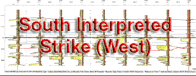
• Cross-sections of the interpreted North-South Dip line, and the two strike lines represented by a Northern Strike Line (split into an Eastern section and a Western Section) and a Southern Strike Line (split into an Eastern section and a Western Section) are provided as potential solutions to this exercise with .pdf files that can be accesses via the thumbnails and .gif or .jpg files from the links provided below. These solutions to the exercises can be printed from either the .pdf, .gif or .jpg images of the figures provided.

As an alternative this cross section can also be viewed as a large .gif file by clicking on the North-South Dip line

As an alternative this cross section can also be viewed as a large .jpg file by clicking on the South Eastern Section

As an alternative this cross section can also be viewed as a large .gif file by clicking on the South Western Section

As an alternative this cross section can also be viewed as a large .gif file by clicking on the South Eastern Section

As an alternative this cross section can also be viewed as a large .gif file by clicking on the South Western Section

• For each of the SP curves (the right trace) the areas of the curve with the "0" or low SP values are inferred to represent shale, while high SP values are inferred to represent sand, i.e. those values further from center line.
• On each of the well logs shale is now colored brown and sand yellow.
• The adjacent well logs are correlated on the basis of similarly shaped curves, by drawing a boundary surface under each correlatable interval. 
• The cross-section is divided into parasequences and the system tracts are identified within each parasequence.  
• The Transgressive Surfaces (TSs) of each parasequence was identified first. These surfaces coincide with thin intervals of winnowed sediment that are produced as the sea transgresses across the underlying sediments. Thus the inferred transgressive surfaces are thin intervals that show a slight increase in grain size over thin shale intervals that may in turn overlie blocky sands. The transgressive surface is often indicated on the SP by an increase in grain size and a coincidental local increase in resistivity which matches carbonate cementation.
• The Maximum Flooding Surfaces (mfs's) of were identified next. On the well logs these surfaces are inferred to coincide with the occurrence of shale (kicks on the logs with the lowest SP values) just beneath sections that coarsen upward (i.e., the SP values increase, exhibiting a vertical funnel shape on the SP log). Three parasequences (each parasequence being enveloped by mfs) were identified and were labelled from the base up as A, B, and C.
• The sequence boundaries (SB) on the cross-sections were the final surfaces identified. These were picked at the base of the channel sands (incised valley fill). A massive boxcar trend in log character was inferred to represent the channel fill of incised valleys and this fill was correlated to adjacent well logs.
• For each parasequence the total sand content in feet (utilize the middle log scale) was estimated while utilizing the middle of the log to mark sand body boundaries and triangles to record changes in grain size within each parasequence). The values were recorded in the spreadsheet.
• Based on the mfs surfaces and the identified channels, the systems tracts for each of the well logs (LST, TST, and HST) were identified.  Channel sands were interpreted to represent a Lowstand Systems Tract which was incised into the underlying Highstand Systems Tract, and is overlain by Transgressive System Tract deposits.  Where no channels were present, the mfs were utitilized to identify the HST (the deposits above the mfs) and the TST (the deposits below the mfs).
• The final step should be to write up an analysis describing your conclusions based on your interpretation of the depositional setting, the evolution of each parasequence and the sand isopach maps..