The
Exercises
The exercises
below involve the analysis of parasequence
using well logs and cores. The parasequences are seperated from
each other using major surfaces that include TS (transgressive
surfaces), mfs (Maximum
Flooding Surface), and SB
(sequence
boundary). This followed by the examination of the stacking
patterns of the parasequences. Finally Fisher diagrams are drawn
to help predict the extent of the bounding and interior surfaces
of parasequences
An analysis of parasequences
should the lead to the interpretation of the depositional settings
of the lithologies that are enveloped by the surfaces listed above.
Finally the parasequence sets can be matched to global sea level
curves in order to identify potential source rocks, reservoirs
and seals. A final product is the definition of "zones"
or "compartments" whose facies are asssociated with
different lithologies which have different characteristics with
different vertical and lateral distributions.
EXERCISES
1- 4
Exercise
1 - Introduction to parasequence identification
Click
on thumb nails to expand images.
Well
# 1 - Shallow shelf region:
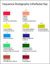
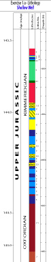 Lithofacies.
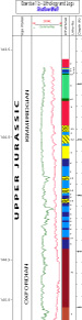 Lithofacies
+ Well Logs.
Lithofacies
+ Well Logs. 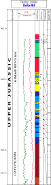 Solution.
Well
# 2 - Deeper region:
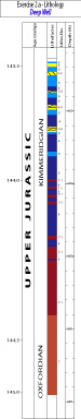 Lithofacies.
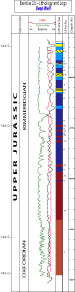 Lithofacies
+ Well Logs.
Lithofacies
+ Well Logs.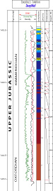 Solution.
If you are confused
in this exercise you should work you way through the earlier sections
of:
1) The Introduction and
2) Parasequence
correlation
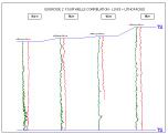
Exercise
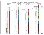
2 - Correlate four well logs on the basis of well logs and cores
used together
Exercise 2
The objective of this exercise is to introduce the concept of
well log correlation. The exercise utilizes the logs of four wells
(right side is north, left side is south). The interval which
is bounded by transgressive surfaces represents a complete sequence
(TS to TS). All wells are datumed to the transgressive surface
(TS) datum at the base of the section. The exercise is subdivided
into two steps:
1. Using the well logs only:
a) For each well, identify the trends in the paleobathymetry and
grain size of the lithology and the logs (shoaling or deepening)
and identify parasequences (cycles) which are bounded by mfs.
b) See if you can find clear electric log events (mainly gamma
log spikes) that can be identified in all or most wells. Use these
markers for correlating all four wells.
c) Determine the overall profile of the section (north to south).
2. By combining the log interpretation with lithofacies cycle
identification, the interpretation process can be much more definite.
a) For each well, identify all cycles.
b) For the overall lithofacies character (shallowing, deepening,
thickness changes, etc.), and in combination with the interpretation
of step 1, identify the third-order sequence major surfaces including
the maximum flooding surface (mfs) and the sequence boundary (SB).
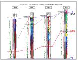
This exercise requires
the identification of the major stratigraphic surfaces that can
be correlated from well to well.
 The surfaces should be identified on the basis of the log character
and the stacking patterns of the wells.
The surfaces should be identified on the basis of the log character
and the stacking patterns of the wells.
 Make
the correlation of the four wells on the basis of parasequences.
Make
the correlation of the four wells on the basis of parasequences.
 Solution.
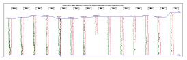
Exercise
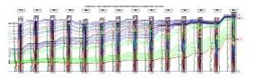
3 - The final and complete regional sequence stratigraphic interpretation
Using the results of
exercise 2, make an interpretation of all fourteen regional wells.
The well spacing is approximately 4 km. The objective of this
exercise is to identify the architecture of the sequence and its
major system tract components (TST, HST, SWM or LST) and to relate
their occurrence to the position of the sea level. The reason
for doing this is to better understand the processes that lead
to the deposition of these different system tracts.
The exercise is subdivided
into two steps:
 Interpretation
based on well logs.
Interpretation
based on well logs.
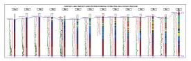 Interpretation
based on lithofacies character + well logs.
Interpretation
based on lithofacies character + well logs.
 Final
Solutoin.
Final
Solutoin.
Exercise
4 - Improve correlation - the use of Fischer Diagrams
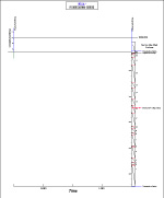
The
Fischer plot is a graph with two axes. The horizontal axis represents
time and the vertical axis represents thickness. Having established
the length of time involved to accumulate the thickness of sediment
within the section a line representing the rate of subsidence
of this section is drawn across the graph from upper left to
lower right, with the upper left end starting at the top of
the section at the time of the initiation of deposition of the
section and the lower right end terminating at the time of the
termination of deposition and at the base of the section.
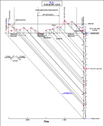
Then working from the base of the section up, plot the thickness
of the first parasequence as a vertical line, with its base
resting on the diagonal subsidence line at the time of the start
of deposition of that parasequence. Now draw a further line
of subsidence from the top of the vertical line representing
the first parasequence to the vertical axis on the lower right.
Next plot the thickness of the second parasequence as a vertical
line, with its base resting on the new diagonal subsidence line
at the time of the start of its deposition. Now plot another
line of subsidence from the top of this parasequence to the
vertical axis on the right. Repeat this process for each of
the parasequences until the vertical lines for each has been
plotted. When this is finished you will note that the subsidence
is represented by a series of inclined parallel lines and the
horizontal spacing of the vertical lines representing the parasequences
is equally spaced. This is because each parasequence is assumed
to have the same time duration. This oversimplification explains
some of the character of this plot.
Now draw a curving line that connects the tops of the each of
the vertical lines representing the thicknesses of each parasequence.
This curve represents sea level position through time. Because
this solution to the exercise is a smooth interpolation, this
curve may it lie just below the crests of some of the parasequences.
However, in this particular case it should not be inferred that
the crests of these parasequences were exposed. Some exposure
has been seen in the local updip stratigraphy but this is ambiguous.
In the case in point the peaks or tops of the parasequences
are mfs, and so might not be expected to show exposure!!! Not
the spacing of the inclined subsidence lines varies. This reflects
variation in the thickness of each parasequence. An increase
in thickness of the parasequences means that accommodation space
was increasing and may be the result of an eustatic rise or
increased subsidence. If the parasequences thin then this means
that there is a decrease in accommodation space and sea level
is falling or subsidence is decreasing.
 Fischer
Diagram cycles mapping.
Fischer
Diagram cycles mapping.
 Fischer
Diagram Solution.
Fischer
Diagram Solution.